Lab 11

Objective

The purpose of this lab was to implement linear feedback control through a simulation in order to balance an inverted pendulum on the back of a virtual robot. This involved taking a naturally non-linear system and controlling it via matrix operations in order to get to a stable point, both in idealized and noisy scenarios.

The Math

Both the inverted pendulum and cart have forces acting on them, as described in the force body diagram below. In our case, the inverted pendulum was affixed to a point on the cart, allowing it to rotate around it, and the cart restricted to a single degree of motion in the +/- x direction. These forces are combined to determine the state vector for the system as a whole.

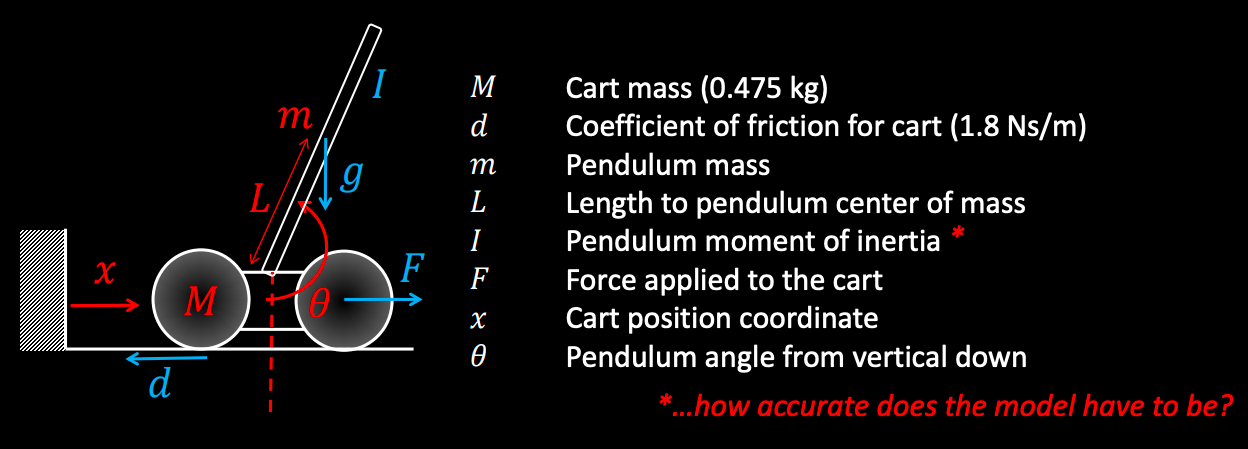
As mentioned before, this is a naturally non-linear system, making it inherently more difficult to determine the control necessary to bring the whole system to a desired state vector. The goal is to linearize the system within the structure of x_dot = Ax+Bu, where A and B are matrices and x and u are column vectors. A describes how the whole system changes over time and is paired with x, the state vector of the system in the form of [x x_dot theta theta_dot]^T. B describes how the whole system will respond to an actuation force, given by u.

The control vector u is linear, equal to -Kx to try and bring the system back to its fixed point by negating its current state in x. This equation can then be substituted into the earlier equation for x_dot, becoming (A - BK)x. This linearly controlled equation has eigenvalues that determine how stable the entire system can be. If these eigenvalues are negative, it leads to system stability (in the case of the inverted pendulum, this means staying upright).

Simulation

We were provided the following Python scripts:

1. pendulumParam.py: initializes physical pendulum parameters and state space equations.
2. pendulumControllerDynamics.py: describes the nonlinear dynamics of the system.
3. signalGenerator.py: computes various reference functions to test the pendulum.
4. pendulumAnimation.py: helper functions for animating the system.
5. plotDataZ.py: helper functions to plot state variables and reference values for debugging.
6. runSimulation.py: integrates the entire vector field using the controller and the true nonlinear dynamics, and plots the results.

The first step to implementing feedback control was to specify the parameters of the robot. The mass was changed to 522g (as recorded in lab 3) and the damping coefficient to 1.8Ns (based on the more realistic value Professor Petersen mentioned).

#Physical parameters of the inverted pendulum known to the controller
m1 = 0.03  # Mass of the pendulum [kg]
m2 = .522  # Mass of the cart [kg]
ell = 1.21  # Length of the rod [m]
g = -9.81  # Gravity, [m/s^2]
b = 1.8  # Damping coefficient [Ns]

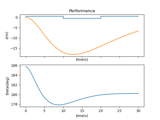
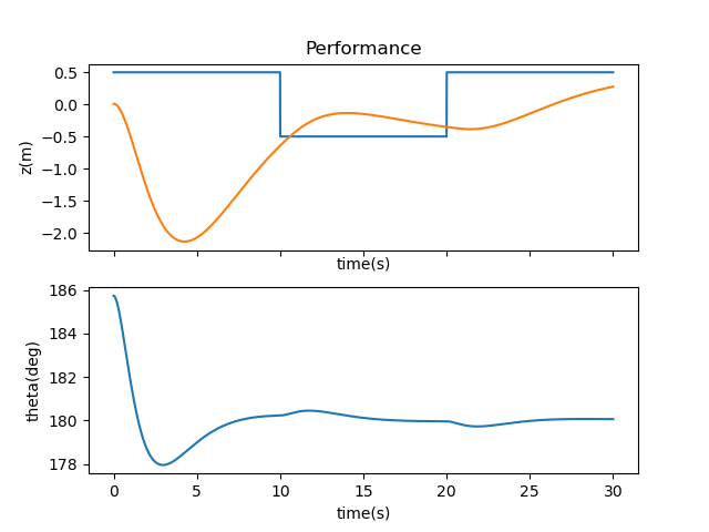
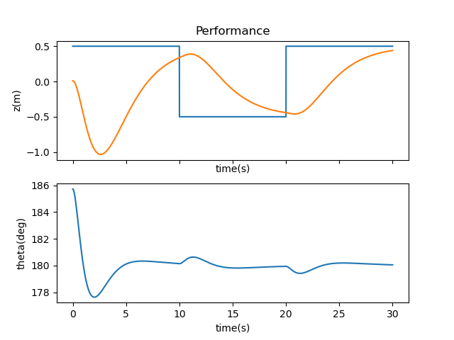
Next came the eigenvalues. Negative eigenvalues ensure a more stable system, but I didn’t know how negative I should go to start. Noting that the eigenvalues shouldn’t be the same, I started with -0.1, -0.2, -0.3, and -0.4. The results are shown in the graph and video below.

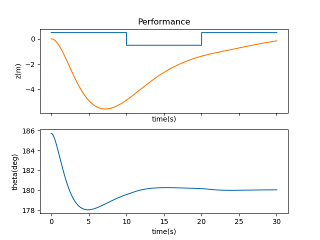
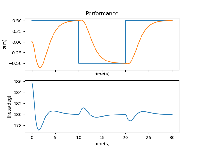
There was for more aggressive control of the system to bring the cart and pendulum back to their fixed position, so I incrementally worked through each eigenvalue, making them more negative until I reached a set of values that relatively stabilized the system. Note that more negative values brought the system closer to its setpoint, rather than fly off the screen. My final eigenvalues were -1.1, -1.2, -1.3, and -1.4, which didn’t lead to a perfectly still system but managed to balance the inverted pendulum pretty well without too large of a range of motion.

This was all specifically accomplished with the following code framework.

 import control
 dpoles = np.array([..insert eigenvalue1.., \
 ..insert eigenvalue2.., \
 ..insert eigenvalue3.., \
 ..insert eigenvalue4..])
Kr = control.place(p.A,p.B,dpoles)
self.u = Kr * (np.subtract(des_state, curr_state))

The A and B matrices were imported from pendulumParam.py. self.u is set to -Kx, where x is the difference between the desired state and the current state. The lack of negation here is due to the order of subtraction between curr_state and des_state; if it were flipped (curr_state - des_state) then there would be a need for a negative sign. A more sophisticated form of feedback control comes in the form of a Linear Quadratic Regulator. This uses two matrices, Q and R, to determine the value of K through the Riccati equation.

#solve algebraic Riccati equation (ARE)
S = scipy.linalg.solve_continuous_are(p.A, p.B, Q, R)
# Solve the Riccati equation and compute the LQR gain
Kr = np.linalg.inv(R).dot(p.B.transpose().dot(S))

Each matrix penalizes changes in the system differently: Q emphasizes changes in the state vector, while R emphasizes changes in the control vector. This was mentioned in lecture as well as in Medium article, this tutorial, and this explanation.

I started first with the following Q and R matrices, and below are its results. The system stabilizes to its setpoint but the motion is unrealistic, switching quickly from sitting still to swaying to one side of the simulation.

Q = np.matrix([[1, 0.0, 0.0, 0.0], [0.0, 1, 0.0, 0.0],
          [0.0, 0.0, 10, 0.0], [0.0, 0.0, 0.0, 100]])
          R = np.matrix([0.001])
          

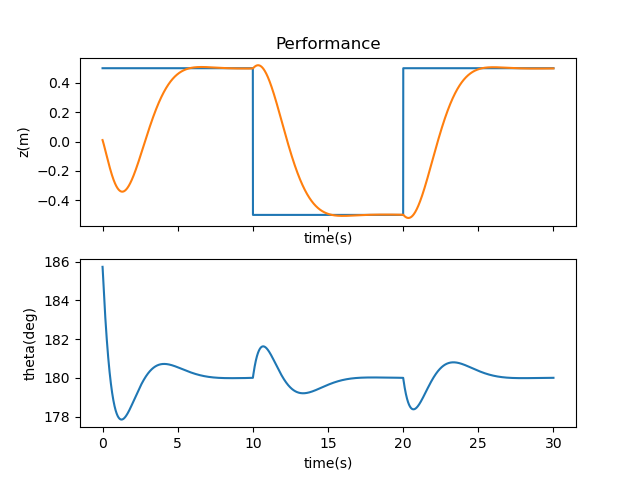
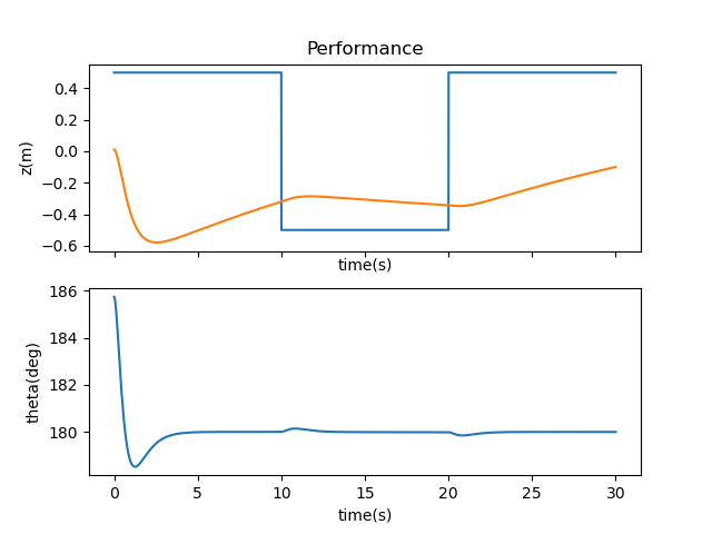
Increasing R to [1000] improved on this front, as it slowed down the balancing motions needed to bring the system back to the setpoint.

On the other hand, decreasing R to 0.0001 exacerbated this problem and combined the slow movements with the quick jerks across the simulation.

Considering the complexity of tuning both Q and R, I chose to keep Q as the same provided matrix and focus my efforts on R (i.e. the control vector). I learned that larger Rs will penalize motion more expensively, hence smaller and slower movements, while smaller Rs will allow the system to move in large swathes with little penalty. With R set to 1000, my eigenvalues were as follows. These seemed reasonable to me, as they were all negative to varying degrees, more so when controlling the theta parameters (as controlling the inverted pendulum is more of a task than the cart).

[-0.01756579+0.j         -3.68824985+0.j         -2.64540865+0.18562646j
          -2.64540865-0.18562646j]
         

A More Realistic Simulation

In this idealized experiment, there is drag and friction but no caps on the potential actuation of the motors. As seen in lab 6 onwards, this isn’t the case with our real robot and therefore had to be taken into account. First there’s deadband, which is the lowest value at which the motors will be able to move the cart. Taking values from lab 3, I calculated this value to be equal to (120 / 255) * (3.33) * (0.522)—120 was the new deadband value I recorded after taping my wheels, 255 was the motor value at which the max acceleration was found, 3.33m/s^2 is the max acceleration from lab 3, and 0.522 is the total mass of the car from lab 3. Saturation is related to this value, expressing the maximum potential force applied by the motors: F = ma = total mass * max acceleration = 0.522 * 3.33. The following code kept u within these boundaries:

if orig_u > 0:
          if orig_u < deadband:
          self.u = np.array([0])
      # elif orig_u > (0.5 * deadband) and orig_u < deadband:
      # self.u = np.array([deadband])
      elif orig_u > saturation:
          self.u = np.array([saturation])
      else:
          self.u = orig_u
else:
      if orig_u > (-1 * deadband):
          self.u = np.array([0])
      # elif orig_u < (-0.5 * deadband) and orig_u > (-1 * deadband):
      # self.u = np.array([-1 * deadband])
      elif orig_u < (-1 * saturation):
          self.u = np.array([-1 * saturation])
      else:
          self.u = orig_u

The original signal generated by this simulation was a square wave; this didn’t jive at all with the conditionals for cutting off at deadband and would crash the simulation. As described by the professor, a vertical signal failed to correct itself due to deadband. The solution for this was to change the signal to that of a sinusoid, therefore never requiring the cart to stand still.

ref = signalGen(amplitude=500, frequency=.5, y_offset=0)
ctrl = pendulumCnt(param=P,zref=ref.sin)

Changing the amplitude and frequency of this sinusoid allowed for my system to work within deadband and saturation to stabilize without crashing.

ref = signalGen(amplitude=160, frequency=0.8,  y_offset=0)  #worked to accommodate deadband
ctrl = pendulumCnt(param=P, zref=ref.sin)

Sensor noise is also abundant in the real world, especially in Klaus. For example, the time of flight sensor had around 2% sigma error in lab 5. To simulate noise, I used a Gaussian distribution called with random.gauss( ) on all four elements of the state vector. I didn’t have time to look into noise on elements other than the x (in this code, z) of the state vector, but I can promise you it exists.

 mu = 0
          sig_z = 0.02
          sig_z_dot = 0.000
          sig_theta = 0.000
          sig_theta_dot = 0.000
          noise = np.array([[random.gauss(mu, sig_z)],
                            [random.gauss(mu, sig_z_dot)],
                            [random.gauss(mu, sig_theta)],
                            [random.gauss(mu, sig_theta_dot)]])
          #print(noise)
          noise_state = np.add(curr_state, noise)
          noise_state[2] = self.limitTheta(noise_state[2])
  

Rather than try to tackle all four noisy variables at once, it was recommended we focus on one. I chose z since I had an error percentage in mind and tuned Q and R with the previously defined sinusoidal signal. Below is my best run with the following matrices and a siq_z of 0.0001 (since 0.02 was too big of a value to tune for):

Q = np.matrix([[3.0, 0.0, 0.0, 0.0], [0.0, 0.5, 0.0, 0.0],
          [0.0, 0.0, 0.5, 0.0], [0.0, 0.0, 0.0, 3.0]])
          R = np.matrix([13000.0
                                 ])