ECE 4960 Fast Robots

Objective

There are many forms of control when looking at any system, including that of an inverted pendulum, and this lab explored one of them: the Kalman filter. Building off of the knowledge of filters and nonlinear systems from the last lab, this was meant to look into a different way of stabilizing the inverted pendulum with the motion of the simulated robot.

Kalman Filter

While the linear quadratic regulator worked over continuous time with matrices Q (to penalize changes in the state vector) and R (to penalize changes in the control vector), the Kalman filter is configured for discrete time systems. This changed the A and B matrices from a continuous form with LQR to a discrete form with the Kalman filter.

The C matrix affects which states are being measured directly and which are being estimated. Every entry is either a 0 or 1; if a row vector contains a 1, that aspect of the state is being measured directly. With the linear quadratic regulator, the C matrix was the following:

C = np.matrix([[1.0, 0.0, 0.0, 0.0], [0.0, 1.0, 0.0, 0.0],
          [0.0, 0.0, 1.0, 0.0], [0.0, 0.0, 0.0, 1.0]])

meaning that all of the states were being measured. For the Kalman filter, the C matrix is:

C = np.matrix([[0.0, 0.0, 0.0, 1.0]])

This shows that the only state being measured is the fourth one, equivalent to the theta dot value.

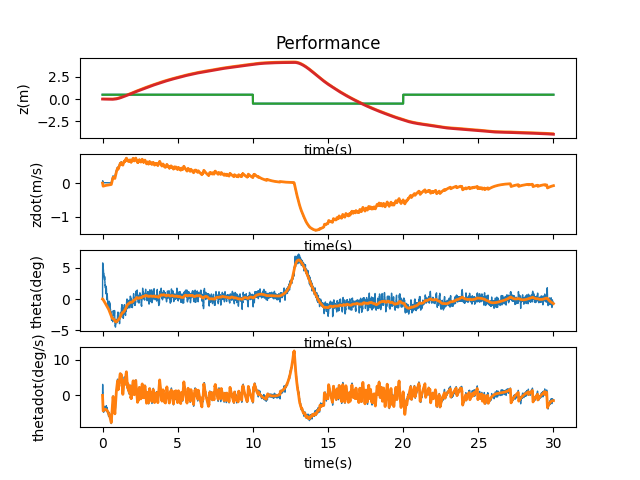
Before I could find out whether or not the A or C matrices were observable, I ran into this error ```AttributeError: 'float' object has no attribute 'sin' ``` when running the runSimulation.py script. Fixing it required changing theta to theta[0] in the np.sin and np.cos calls in runSimulation and pendulumAnimation. Once that was out of the way, I got the following behavior:

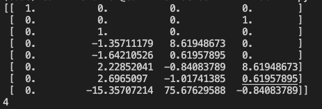
To see whether or not the state is observable, I printed control.obsv(P.A,P.C):

The first column vector contains all zeros showing that the matrix is rank deficient. This was emphasized when printing the value of np.linalg.matrix_rank(control.obsv(A,C)) and seeing it was 3. This means that not all states within the system matrix are observable.

Adding Realistic Noise

There are many potential sources of noise within the system. With this program we focused on adding process (sigma_u) and measurement (sigma_n) noise to test the robustness of the filter. pendulumNonlinearDynamics had a line commented out that added a random amount of noise.

dydt = [ydot0 + np.random.randn()*0.01, ydot1 + np.random.randn()*0.01, ydot2 + np.random.randn()*0.01, ydot3 + np.random.randn()*0.01]

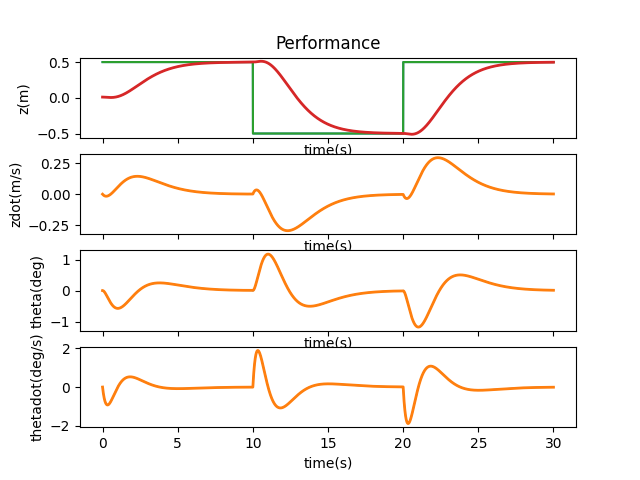
There was some sway of the system, but overall the inverted pendulum was able to right itself without too much movement. Unfortunately, real-world systems also tend to have a good amount of sensor noise, so I had to add some random amount of noise at every timestep. The loop on t_array within runSimulation accomplishes this, and within it the variable y_kf takes the dot product of the previous state vector and the C matrix before being used in the Kalman filter. Therefore I added np.random.randn() to this value, which added a value from a Gaussian)distribution of mean 0 and variance 1. This caused the system to act as such:

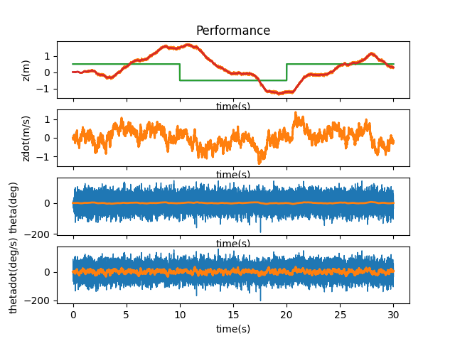
I changed this to y_kf = P.C.dot(old_state) + np.random.randn() * 0.01 to match the same range of noise as process noise. The resulting behavior was as such:

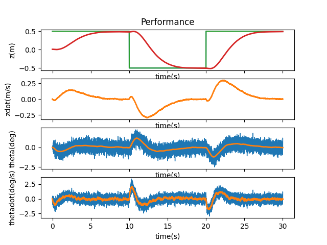
Adding Discrepancy to the Initial State

The initial state of the system is the initial values for each aspect of the state vector when the system first runs. Originally this was defined as mu = np.array([[P.z0], [P.zdot0], [P.theta0], [P.thetadot0]]). Considering the level of process and measurement noise I added previous, first I added 0.01 to each term of the initial state. This didn’t affect the behavior of the system much:

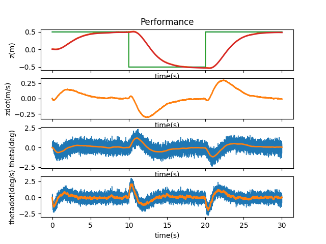
I took things a step further by increasing the magnitude of the added factor by 10 (to 0.1). This seemed to be a value that wouldn’t make too large an impact on each of the aspects of the state vector (since the ranges for their values could easily absorb it, i.e. -2 to 2 for z).

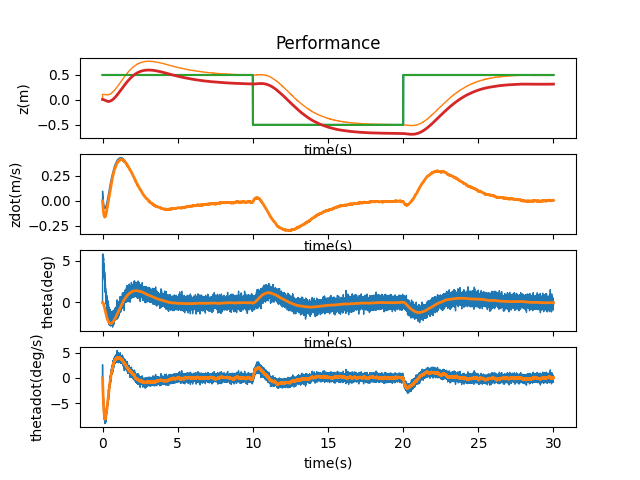
I wanted to see how far I could push it when adding to the initial state before the Kalman filter was overwhelmed. Following the trend of increasing by an order of magnitude, I added 1 and saw the cart promptly run off the side of the screen, eventually coming back to stabilize:

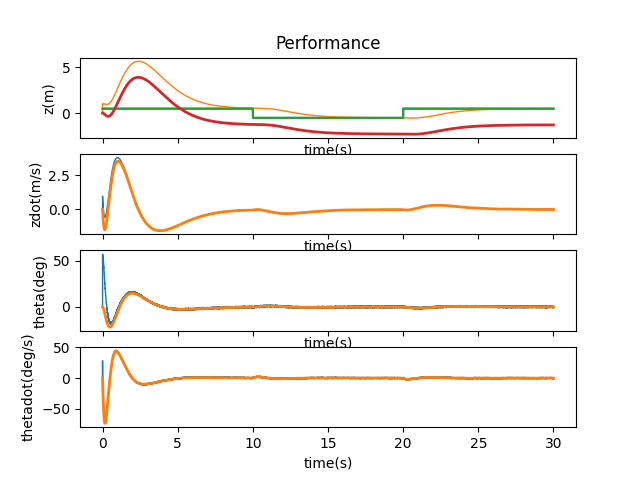
Performing a binary search between 1 and 0.1, I added 0.5 and the cart didn’t run off the screen.

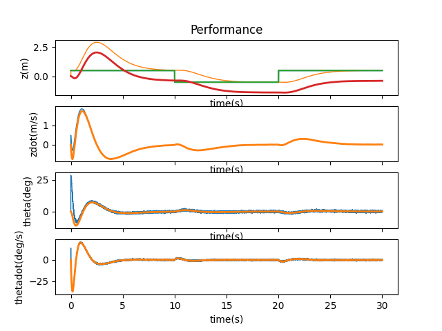
However, I decided to stick with 0.1 since 0.5 would have jerky motion every now and then.

Saturation and Deadband

Lab 11 involved adding boundaries on the motion of the system using saturation and deadband values calculated with numbers about the real robot from earlier labs.

deadband = (120 / 255) * (3.33) * (0.522)  #~0.8 = deadband of robot/motorval (from lab 6) * acc * mass
          saturation = 0.522 * 3.33

From that experience, I knew I had to find the control vector u and perform a series of conditional statements on it in order to bound check around the saturation and deadband values. u was within the t_array loop in runSimulation, equal to u = -Kr.dot(mu - des_state). I implemented the following code after that expression:

if u > 0:
            if u < deadband:
            u = 0
          elif u > saturation:
            u = saturation
          else:
          if u > (-1 * deadband):
            u = 0
          elif u < (-1 * saturation):
            u = -1 * saturation

Here is what the simulation looked like after adding this code. Unlike the LQR filter, no additional tweaks had to be made for the system to stabilize.

Changing the A and B Parameters

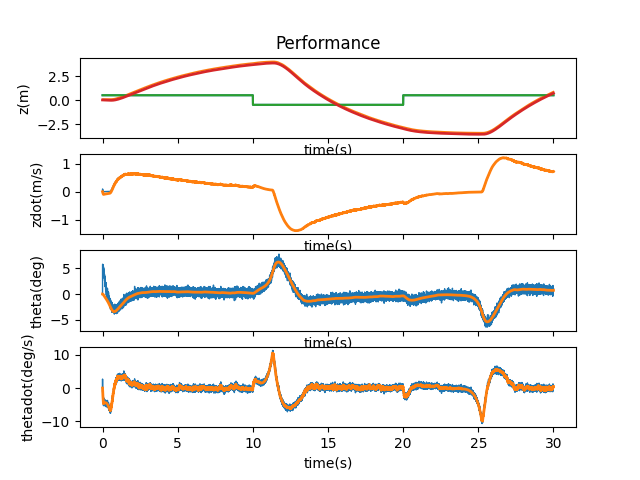
At first, the A and B matrices were set to the following:

A = np.matrix([[0.0, 1.0, 0.0, 0.0],
                      [0.0, -b/m2, -m1*g/m2, 0.0],
                      [0.0, 0.0, 0.0, 1.0],
                      [0.0, -b/(m2*ell), -(m1+m2)*g/(m2*ell), 0.0]])
            B = np.array([[0.0], [1.0/m2], [0.0], [1.0/(m2*ell)]])

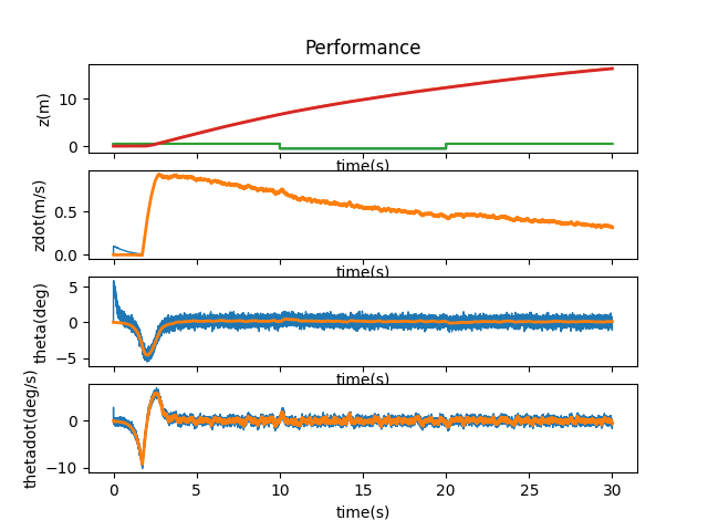
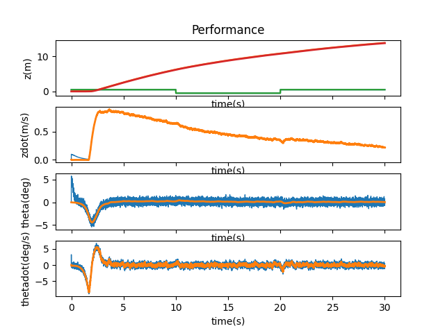
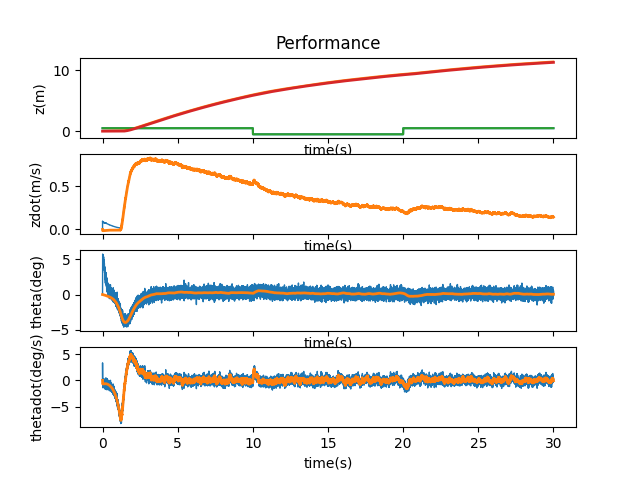
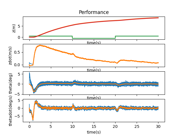
I went through a lot of adjustments with these matrices to see how they each would react when changed individually and changed together. When looking at the first coefficient of 1.01, the three combinations of A and B being affected all ended up stabilizing. However, when both matrices were multiplied by the coefficient, the system was smoother in its motions—A took longer to stabilize, while B was jerkier in its motions.

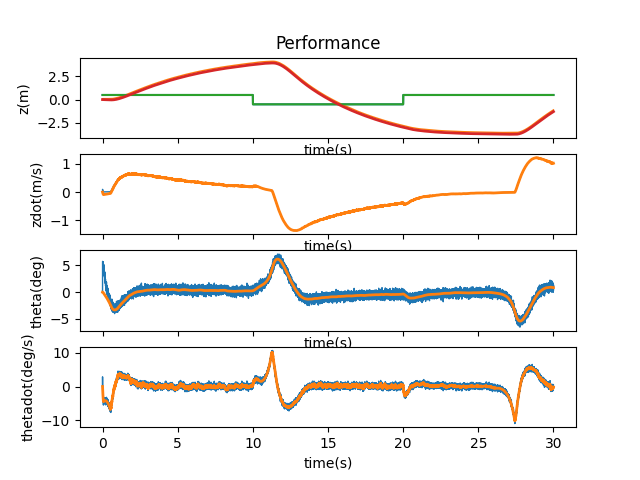
A * 1.01

B * 1.01

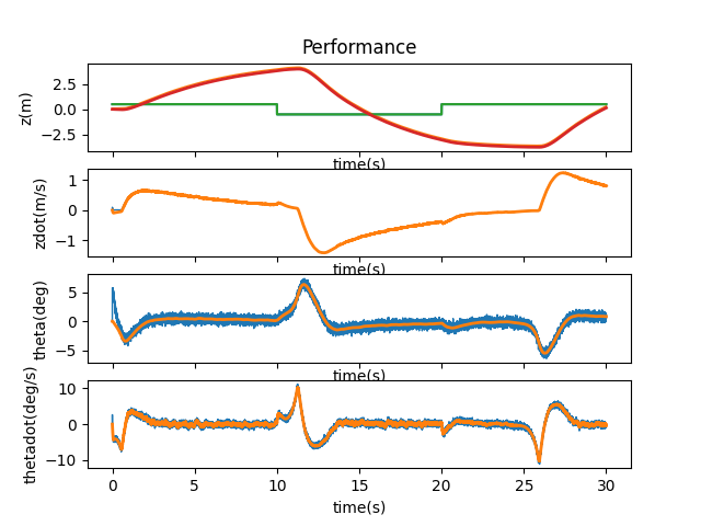
A and B * 1.01

I then checked out 1.5, 1.4, 1.3, 1.2, 1.1, 1.05, 1.03, and 1.02 to find the maximum bound that A and B could be manipulated by. After 1.2, the cart ran off the side of the simulation and didn’t come back to stabilize itself. A multiplier of 1.03 seems to be the max boundary for the system to come back and stabilize itself, but it does have slight jerkiness to its movements.

A and B * 1.5

A and B * 1.4

A and B * 1.3

A and B * 1.2

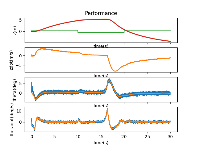
A and B * 1.1

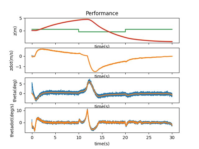
A and B * 1.05

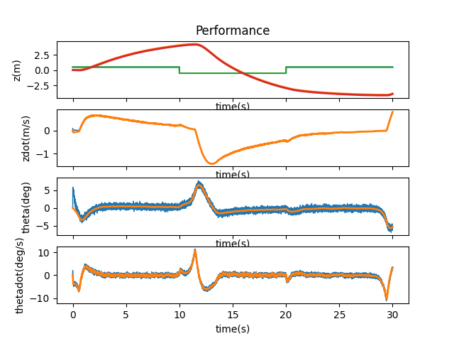
A and B * 1.03

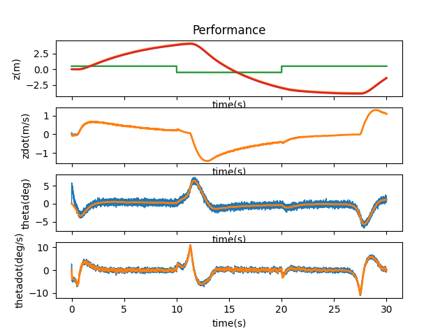
A and B * 1.02

Changing Update Time

The initial value for the update time (found in pendulumParam) was 0.001. Sticking with the trend of making changes by factors of 10, I increased the update time to 0.01 and saw a stable response.

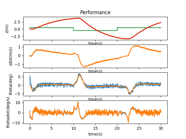
Another jump to 0.1 didn’t show that same stability.

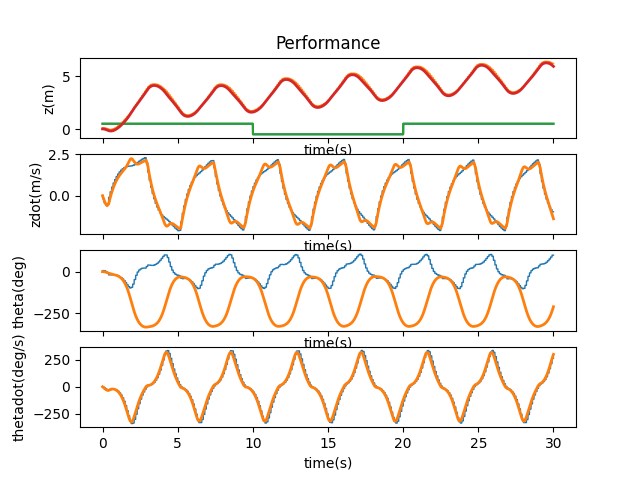
A binary drop to 0.05 was still stable, so I continued working my way via 0.01 increments to find the point at which the system loses its stability. I found this to be at 0.07.

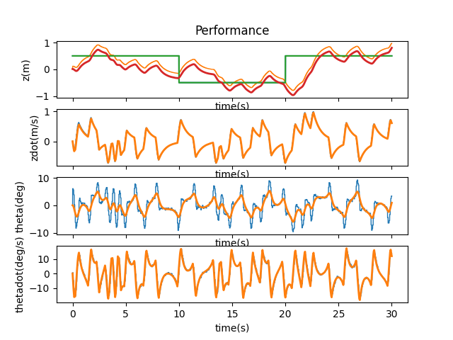
T = 0.05

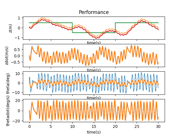
T = 0.06

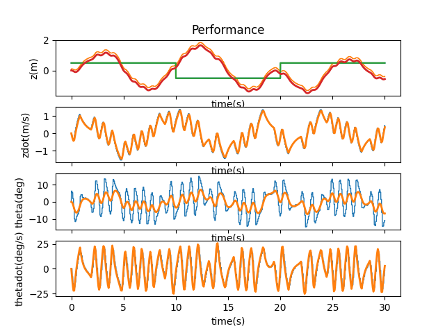
T = 0.07

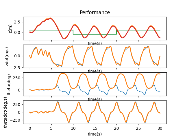
T = 0.08

Comparison to Klaus

As I’ve said before, Klaus is chock full of his own little quirks and disadvantages; therefore, I do believe that this simulation is relatively accurate to how a real-world implementation would play out. With regards to noise, the values of my time of flight sensors were never good enough for perfect localization and my motors weren’t evenly calibrated for all surfaces. The motors also had their own mechanical constraints due to deadband caused by friction (especially without the tape on his wheels). When sending data over the Bluetooth connection, time to respond was slowed down considerably. I don’t think my configurations in the virtual space would match Klaus perfectly, but they’d definitely imitate a more realistic version of my interactions with my hardware.

Extra Credit: Frequency of Measurements

Sensors by nature will not read at the same frequency for various reasons (i.e. range, accuracy, noise). To simulate this, thetadot was changed to be measured at a frequency of 100Hz and z to be measured at a frequency of 10Hz. First the C matrix was adjusted to directly measure both z and thetadot (the first and fourth state vectors).

C = np.matrix([[1.0, 0.0, 0.0, 0.0],[0.0, 0.0, 0.0, 1.0]])

The measurement noise added to y_kf from earlier was changed from np.random.randn() * 0.01 to np.random.randn(2, 1) * 0.01 so as to add an array of randomized noise.

To change the frequency of reading measurements, I added the following function to kalmanFilter.py and imported it into runSimulation.py. It uses a counter variable (implemented as t from the t_array loop in runSimulation.py) to see if it’s a multiple of 10, to then update z and thetadot, otherwise just update thetadot.

def kalmanFilterEC(mu, sigma, u, y, i):
    if i % 10 == 0:  #frequency = 10Hz, for both thetadot, z
    C_KF = P.C
    y_KF = y
else:  #frequency = 100Hz, only for thetadot
    C_KF = P.C[1, :]
    y_KF = y[1, :]

mu_p = Ad.dot(mu) + Bd.dot(u)
sigma_p = Ad.dot(sigma.dot(Ad.transpose())) + sigma_u

y_m = y_KF - C_KF.dot(mu_p)
sigma_m = C_KF.dot(sigma_p.dot(C_KF.transpose())) + sigma_n
kkf_gain = sigma_p.dot(C_KF.transpose().dot(np.linalg.inv(sigma_m)))

mu = mu_p + kkf_gain.dot(y_m)
sigma = (np.eye(4) - kkf_gain.dot(C_KF)).dot(sigma_p)

return mu, sigma

Here is the result of this change in the rate of measurement. The system takes a little bit longer to stabilize and stays off screen for a bit longer than before, but still works! The major pro here is that the system matrix is now observable since it has a rank of 4.

Lab 12