Lab 7
Grid Localization using Bayes Filter and Mapping
In a switch up, this week started with the virtual environment. During lecture we’ve spent a good amount of time learning about probability, whether in the context of noisy sensors or predicting position. This lab ramps up to building our own Bayes filter by emphasizing the pseudocode necessary to complete each step.
Code was provided that established the robot and a new virtual environment, then controlled the robot to navigate this environment. The video below shows the robot moving around obstacles as its odometry and ground truth readings are plotted.
Below is the pseudo code written after the code to execute the motion of the robot. This is meant to serve as a guide for the actual implementation of a Bayes Filter. We were able to extend any of the functions to incorporate other parameters or add helper functions.
# In world coordinates
        def compute_control(cur_pose, prev_pose):
        """ Given the current and previous odometry poses, this function extracts
            the control information based on the odometry motion model.

            Args:
                cur_pose  ([Pose]): Current Pose
                prev_pose ([Pose]): Previous Pose

            Returns:
                [delta_rot_1]: Rotation 1  (degrees)
                [delta_trans]: Translation (meters)
                [delta_rot_2]: Rotation 2  (degrees)
            """
        delta_x = cur_pose[0] - prev_pose[0] #this is equal to the amount of translational change in x
        delta_y = cur_pose[1] - prev_pose[1] #this is equal to the amount of translational change in y
        delta_yaw = cur_pose[2] - prev_pose[2] #this is equal to the amount of rotational change in yaw

        delta_rot_1 = Math.tan(delta_y/delta_x) #angular change due to a change in position is equal to tan of change in y/change in x
        delta_trans = Math.sqrt((delta_x ** 2) + (delta_y ** 2)) #distance between two points
        delta_rot_2 = delta_yaw + delta_rot_1 #pre-calculated change in yaw

        return delta_rot_1, delta_trans, delta_rot_2

        # In world coordinates
        def odom_motion_model(cur_pose, prev_pose, u):
        """ Odometry Motion Model

            Args:
                cur_pose  ([Pose]): Current Pose
                prev_pose ([Pose]): Previous Pose
                (rot1, trans, rot2) (float, float, float): A tuple with control data in the format
                                                           format (rot1, trans, rot2) with units (degrees, meters, degrees)


            Returns:
                prob [float]: Probability p(x'|x, u)
            """
        #This is an implementation of the Bayes filter following the Markov assumption on state x_t (cur_pose)
        #Transition probability/action model for the prediction step
        #It specifies how the robot state evolves over time as a function of robot controls u_t
        #p(x'|x,u) = (p(x,u | x') * p(x')) / (p(x,u)) = eta * p(x,u | x') * p(x')

        computed_control = compute_control(cur_pose, prev_pose);
        delta_trans = computed_control[0];
        delta_rot_1 = computed_control[1];
        delta_rot_2 = computed_control[2];


        #calculate probability of each condition
        prob1 = loc.gaussian(delta_trans, u[0], loc.odom_trans_sigma);
        prob2 = loc.gaussian(delta_rot_1, u[1], loc.odom_rot_sigma);
        prob3 = loc.gaussian(delta_rot_2, u[2], loc.odom_rot_sigma);

        prob = prob1*prob2*prob3;

        return prob

        def prediction_step(cur_odom, prev_odom):
        """ Prediction step of the Bayes Filter.
            Update the probabilities in loc.bel_bar based on loc.bel from the previous time step and the odometry motion model.

            Args:
                cur_odom  ([Pose]): Current Pose
                prev_odom ([Pose]): Previous Pose
            """
        u = compute_control(cur_odom, prev_odom) #finding the control information of the robot
        prob = odom_motion_model(cur_odom, prev_odom, u) #finding the probability of p(x'|x,u), state transition probability
        loc.bel_bar = prob * loc.bel

        def sensor_model(obs, u):
        """ This is the equivalent of p(z|x).


            Args:
                obs ([ndarray]): A 1D array consisting of the measurements made in rotation loop

            Returns:
                [ndarray]: Returns a 1D array of size 18 (=loc.OBS_PER_CELL) with the likelihood of each individual measurements
            """
        #Calculating measurement probability
        #It specifies how the measurements are generated from the robot state x_t
        #p(z|x) = p(x|z) * p(z) / p(x) = eta * p(x|z) * p(z)
        prob_array = []
        for z in obs:
            prob_array.append(loc.gaussian(obs[i], u, loc.sensor_sigma))

        return prob_array

        def update_step(eta, obs, u):
        """ Update step of the Bayes Filter.
            Update the probabilities in loc.bel based on loc.bel_bar and the sensor model.
            """
        prob = sensor_model(obs, u)
        loc.bel = eta * prob * loc.bel_bar
Last lab centered around establishing a smooth continuous rotation around the z axis by using a PID feedback control loop. That kind of steady motion is extremely useful in the context of an environmental scan, when large amounts of data can be gathered from various sensors in order to better visualize the robot’s surroundings.
Unfortunately for me, my floor isn’t one that’s conducive to smooth, controlled turning on Klaus’s axis. My PID code worked, but only on the seat of a wooden chair. Rather than let the chair block the sensor and corrupt the readings, I opted for manual turning of the robot. I made sure to keep the center of the robot as centered on the coordinates in question as possible, in addition to taking note of the orientation of Klaus so I wouldn’t accidentally move in front of the sensors.
I decided to use my kitchen as my environment due to its relatively even lighting and its smoother floor (which is possible for Klaus to move on normally, but unfortunately not rotate). My kitchen feeds directly into my living room, so in an effort to restrict the space and give it a more interesting definition, I walled it off with cardboard boxes and added a cooler as a peninsula.
It took trial and error to develop an environment that Klaus could adequately detect. At first, when the kitchen was open and no obstacles were added, the data didn’t show any right angles and even sometimes missed entire walls.
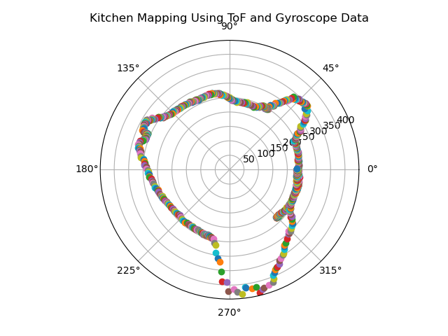
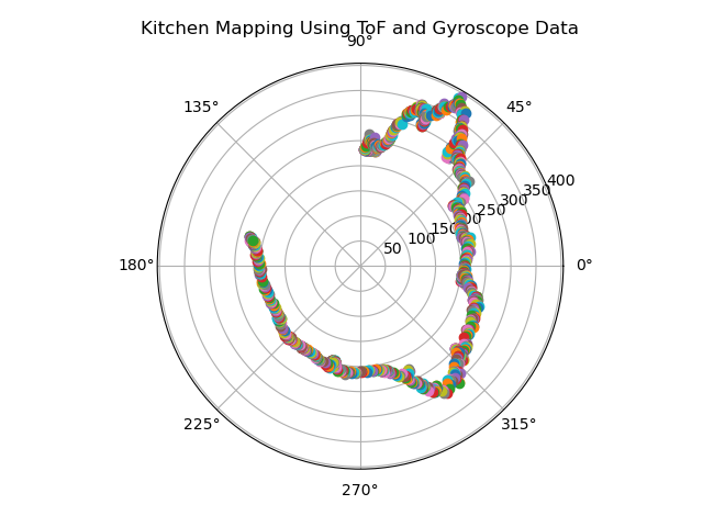
As a sanity check, I placed Klaus in a pen constructed of three cardboard boxes and my refrigerator in order to see what data in a very constricted space would look like. Though still not perfectly straight, the walls of the boxes were more defined. Something to note is the reflectivity of my white refrigerator, which may have affected the sensor readings (particularly when Klaus was facing the fridge head on).


Once the final environment was set up, I did two successive manual scans of the kitchen from the middle of the area. To reduce the time spent plugging and unplugging Klaus to my laptop, data was sent via a Bluetooth bytestream. The focus was on data from the time-of-flight sensor and gyroscope, but all raw sensor data was sent in a large packet array so as to back up their readings. I used this resource to ensure that each of my packets were unpacked properly.
if (bytestream_active)
              {
                counterTransmit++;
                if (counterTransmit>=20) {
                  t0 = micros(); // start time

                  if( myICM.dataReady() ){
                    myICM.getAGMT();

                    // PITCH
                    pitchAcc = getPitchAcc(myICM.accX(),myICM.accZ());
                    pitchAccLPF = applyLPF(pitchAcc, prevPitchAcc, 0.2);
                    prevPitchAcc = pitchAccLPF;
                    pitchGyr = getPitchGyr(pitchGyr, myICM.gyrY());
                    pitchFusion = (prevPitchFusion + pitchGyr * dt/1000000) * (1-alpha) + pitchAccLPF * alpha;
                    prevPitchFusion = pitchFusion;

                    // ROLL
                    rollAcc = -getRollAcc(myICM.accY(),myICM.accZ()); //flipped sign to be consistent with gyroscope data
                    rollAccLPF = applyLPF(rollAcc, prevRollAcc, alpha);
                    prevRollAcc = rollAccLPF;
                    rollGyr = getRollGyr(rollGyr, myICM.gyrX());
                    rollFusion = (prevRollFusion + rollGyr * dt/1000000) * (1-alpha) + rollAccLPF * alpha;
                    prevRollFusion = rollFusion;

                    // YAW
                    yawGyr = getYawGyr(yawGyr, myICM.gyrZ());
                    xMag = myICM.magX()*cos(pitchGyr*M_PI/180)-myICM.magZ()*sin(pitchGyr*M_PI/180);
                    yMag = myICM.magY()*sin(pitchGyr*M_PI/180)*sin(rollGyr*M_PI/180)-myICM.magY()*cos(rollGyr*M_PI/180)+myICM.magZ()*cos(pitchGyr*M_PI/180)*cos(rollGyr*M_PI/180);
                    yawMag = atan2((myICM.magX()*cos(pitchFusion) + myICM.magZ()*sin(pitchFusion)), (myICM.magY()*cos(rollFusion) + myICM.magZ()*sin(rollFusion)));

                    distance = distanceSensor.getDistance(); //Get the result of the measurement from the ToF sensor
                    proxValue = proximitySensor.getProximity();  //Get result from prox sensor
                    distanceSensor.clearInterrupt();

                    Serial.print(micros());
                    Serial.print(", ");
                    Serial.print(distance);
                    Serial.print(", ");
                    Serial.print(proxValue);
                    Serial.print(", ");
                    Serial.print(pitchFusion);
                    Serial.print(", ");
                    Serial.print(rollFusion);
                    Serial.print(", ");
                    Serial.print(yawGyr);
                    Serial.print("\n");

                    res_cmd->command_type = BYTESTREAM_TX;  //set command type to bytestream transmit
                    res_cmd->length = 26;                    //length doesn't matter since the handler will take care of this
                    //TODO: Put an example of a 32-bit integer and a 64-bit integer
                    //for the stream. Be sure to add a corresponding case in the
                    //python program.
                    //Serial.printf("Stream %d \n", bytestream_active);

                    // pack up data to send
                    unsigned long t=micros(); //send current time for x axis
                    memcpy(res_cmd->data, &t, 4);
                    memcpy(res_cmd->data+4, &distance, 4);
                    memcpy(res_cmd->data+8, &proxValue, 4);
                    memcpy(res_cmd->data+12, &pitchFusion, 4);
                    memcpy(res_cmd->data+16, &rollFusion, 4);
                    memcpy(res_cmd->data+20, &yawGyr, 4);
                    amdtpsSendData((uint8_t *)res_cmd, 26);  //2 bytes for type and length, 14 bytes of data
                  }else{
                    Serial.println("Waiting for data");
                    delay(500);
                  }
                    counterTransmit = 0;
                }
                //Print time
                unsigned long t = micros();
                Serial.printf("Packet %d sent at %d micro seconds \n", packet_count, t);
                packet_count++;
              }
This data was plotted with the following code:
import numpy as np  #used for generating arrays
          import matplotlib.pyplot as plot  #used for graphs to visualize data
          from scipy import pi
          from scipy.fftpack import fft  #used for the fft algorithm
          import pandas as pd
          import csv
          import math

          r = []
          theta = []

          plot.axes(projection='polar')

          with open('tmp.csv', 'r') as csv_file:
              next(csv_file)
              csv_reader = csv.reader(
                  csv_file)  # Making use of reader method for reading the file
              for line in csv_reader:  #Iterate through the loop to read line by line
                  r.append(float(line[9]))
                  t = math.radians(float(line[13]))
                  theta.append(t)

          # Set the title of the polar plot
          plot.title('Kitchen Mapping Using ToF and Gyroscope Data')

          for i in range(0, len(theta)):
              plot.polar(theta[i], r[i], 'o')

          # Display the Polar plot
          plot.show()
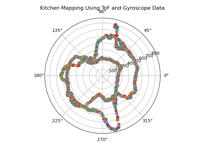
The first scan is more true to the actual shape of the kitchen. Reasoning for the inaccuracy of the second scan is the inherent jerkiness of the wheels; even when being moved manually, the wheels have a good amount of traction, which may have skewed the sensor data at some and therefore propagated that error throughout the scan. Additionally, as will be made more clear later, the ToF sensors aren’t very reliable. One theory is that the reflectivity of the gray flooring may be interfering with the sensing capabilities of the ToF sensor. It also may be an issue of resolution in that the walls of the space may be too far away for the sensor to give accurate, granular readings of distance.
Referencing work from Daniel DiAngelis and Katie Bradford, I tried two different transformation matrices to convert my data from the polar coordinate system to my world coordinate system. There were mixed results.
My first attempt centered around the following equation, which describes that the position in the world coordinate frame is equal to the product of the transformation matrix from the world frame to the robot frame, the transformation matrix from the robot frame to the sensor frame, and the position of the robot via sensor readings.

theta = -yaw*pi/180;
          distance = tof;
          x = zeros(1, length(theta));  % vector for x values
          y = zeros(1, length(theta));  % vector for y values
          for k=1:length(theta)  % for each measurement
              pos_sensor = [distance(k); 0; 1];
              robot2world = [cos(theta(k)) -sin(theta(k)) xR;
                            sin(theta(k))  cos(theta(k)) yR;
                            0            0           1 ];
              sensor2robot = [1 0 63.5;
                              0 1 12.7;
                              0 0 1 ];
              pos_world = robot2world*sensor2robot*pos_sensor;
              x(k) = PW(1);
              y(k) = PW(2);
          end
For the matrix from robot to sensor frame, I determined the sensor to be offset from the center of the robot (the point at which rotations were made) to be 63.5mm in the x direction and 12.7mm in the y direction. This was taking into consideration the coordination axes of the ToF sensor.
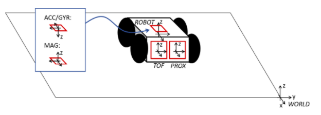
xR and yR then became the coordinates of the robot at each manual scan. The coordinates had to be converted into mm, taking into consideration the offset of the origin from the corner of the room (since I couldn’t shove Klaus into a corner). With that scenario, the following graph was plotted, with the outline of the space plotted for reference:
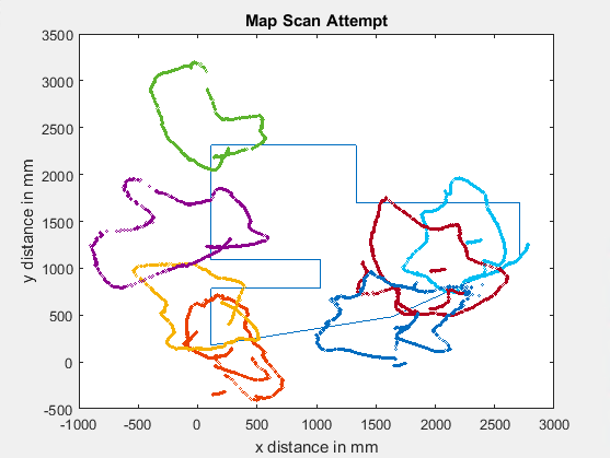
This data was confusing because each set seemed similar to the shape of the areas, but was incorrect with regards to orientation and scaling. With this in mind, I experimented with setting xR and yR to be the coordinates of the origin (xR = 114.3, yR = 177.8) and ended up with a more reasonable looking plot. However, I was uneasy about the reasoning for setting xR and yR to the origin.
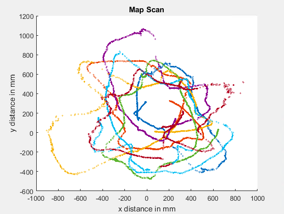
That’s when I decided to try out a rotational matrix around the z axis, exactly the movement Klaus was performing for the scan. This was explicitly offset by the coordinates defined for the origin, 114.3 and 177.8

heta         = yaw;
          theta_radians = deg2rad(theta);
          r             = tof;

          x_data = zeros(1, length(r));
          y_data = zeros(1, length(r));
          for i = 1:length(r)
              r_matrix = [r(i); 0; 1];
              rotation_matrix = [cos(theta_radians(i)) -sin(theta_radians(i)) 0; sin(theta_radians(i)) cos(theta_radians(i)) 0; 0 0 1;];
              new_matrix = rotation_matrix*r_matrix;
              x_data(i) = (new_matrix(1)-114.3);
              y_data(i) = (new_matrix(2)-177.8);
          end
The plotted data has more of a resemblance to the shape of the environment, but there are residual issues with the orientation of the data. Similar to my original issue with transformation matrices, each dataset performs a scan that looks like the room, but the angle at which it’s oriented depends on the initial coordinates. I didn’t have time to debug it but that leads me to believe there needs to be more filtering for the gyroscope.
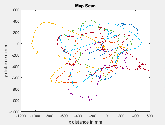
If there was a constraint on the number of readings that could be taken, the readings at every angle could be averaged. Especially as the robot spends more time in a specific position and orientation, the readings reach a sort of steady state and can be more reliable, in addition to less wasteful in terms of space.
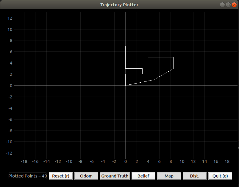
After drawing out the environment by hand, I was able to determine the start and end coordinate arrays pretty easily.
# Start points for each line segment describing the map
          start_points = np.array([[0, 0],
          [0,2],
          [3,2],
          [3,3],
          [0,3],
          [0,7],
          [4,7],
          [4,5],
          [8.5,5],
          [8.5,3],
          [5,1]])

          # End points for each line segment describing the map
          end_points = np.array([  [0,2],
          [3,2],
          [3,3],
          [0,3],
          [0,7],
          [4,7],
          [4,5],
          [8.5,5],
          [8.5,3],
          [5,1],
          [0,0]])
Plotting in the virtual machine resulted in the following shape:
